

SciMethods: Using a Scientifica Multiphoton SliceScope for Fluorescence Lifetime Imaging
Kim Doré1, Jonathan Aow1, Roberto Malinow1, Christian Wilms2
1 Department of Neuroscience and Section for Neurobiology, Division of Biology, Center for Neural Circuits and Behavior, University of California, San Diego, USA;
2 Scientifica Ltd., Uckfield, UK
Introduction
Fluorescence microscopy – particularly two-photon microscopy – has revolutionised neuroscience research over the past two decades. In particular, imaging of live cells and tissue has pushed our understanding of the functioning of the brain on levels ranging from single proteins over local circuits to whole brain areas1. The vast majority of fluorescence microscopy users measure variations of the intensity (i.e. brightness) or colour (i.e. wavelength) of fluorescence over space or time to create an image or movie. A third characteristic of fluorescence is used much less frequently: the fluorescence lifetime. Defined as the average time a fluorescent molecule remains in the excited state before emitting a fluorescent photon (Figure 1A), this lifetime contains a wealth of quantitative information on the excited molecule itself as well as its immediate environment (e.g. pH, ion concentration, solvent polarity). Thus, fluorescence lifetime imaging microscopy (FLIM) adds another layer of information to fluorescence imaging by measuring the fluorescence lifetime in each pixel of a microscopic image.
To determine the fluorescence lifetime of a fluorophore, the time between the excitation pulse and the fluorescence emission is measured for each fluorescent photon. Repeating this time measurement for thousands of detected photons leads to a “photon arrival time” histogram. The time-course of this histogram is the time-course of the measured fluorescence decay. Because the timing of each photon is measured and assigned to that photon, this technique is referred to as “time-correlated single photon counting” (TCSPC, Figure 1B)2. In two-photon imaging, only a small fraction of excitation pulses results in the detection of a fluorescent photon. This enables both PicoQuant and Becker & Hickl to use a so-called reverse start-stop measurement to increase the efficiency of the TCSPC measurement. In this mode, the detected photon starts the timer, and the next excitation pulse stops it.
A FLIM system will store the fluorescence decay histograms for each pixel, allowing the fluorescence lifetimes to be analysed pixel by pixel. As the sum of all photons detected at each pixel is the fluorescence intensity, a FLIM system also provides full access to intensity imaging data. Thus, each data set can be analysed for both fluorescence lifetime and intensity, allowing the complete information acquired in the experiment to be used.
Fluorescence lifetime is a sensitive reporter of a fluorescent molecule’s environment. In addition, it is insensitive to changes in the excitation intensity, the volume of the sample in focus, or the fluorophore concentration. FLIM can thus be used to quantify numerous aspects of cellular function, without needing to take such experimental variations into detailed consideration. Common applications in neuroscience include measuring intracellular chloride concentrations3 or measuring intracellular calcium concentration4. But one of the most versatile uses of FLIM in the past decade has been the precise measurement of molecular interactions using Förster Resonance Energy Transfer (FRET)5.
FRET occurs when the emission and excitation spectra of two very closely spaced fluorophores overlap. If both of these spectral and the spatial criteria are met, excitation of a donor fluorophore will result in fluorescence emission by an acceptor fluorophore. The efficiency of this energy transfer from donor to acceptor is strongly dependent on the distance between the two. For FRET to be detectable at all, an inter-fluorophore distance in the single digit nanometre range is required. This distance range is ideal for determining the interaction of proteins as their size is typically around 2-10nm (e.g. receptor subunits and associated proteins)6 or changes in the confirmation of larger proteins and protein complexes (e.g. ion channels)7. To measure the interaction between two proteins, they are linked to fluorophores that have been spectrally matched for high potential FRET efficiency (so-called FRET-pairs e.g. CFP-YFP or GFP-RFP). Having done this, it is possible to observe FRET if the proteins are indeed interacting.
Commonly FRET is measured by acquiring a series of images in different combinations of excitation and emission channels. This approach has the disadvantage of being slow and error-prone8,9. On the other hand, FRET has the effect of shortening the donor’s fluorescence lifetime by adding an alternative route for the fluorophore to return to the ground state (Figure 1C). Thus, using a detailed analysis of the fluorescence lifetime, it is possible to determine both the distance between interacting fluorophores as well as the fraction of interacting molecules from a single measurement of the donor fluorescence lifetime10.
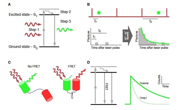
Figure 1: Basic principles of fluorescence lifetime. A: Jablonksi diagram showing the electronic processes during two-photon excited fluorescence. Step 1 is the promotion of an electron from the ground state to the first excited state. Step 2 is the vibrational relaxation within the first excited state. Finally, step 3 is the return of the electron to the ground state under emission of a fluorescent photon. B: Principle of TCSPC. Some laser pulses (top, red) result in the emission of a fluorescent photon (green). The time between the excitation pulse and photon emission is measured and added to a timing histogram (bottom left). After collecting timing information for thousands of photons an exponential function can be fit to the resulting histogram (bottom right). C: FRET between two fluorescence proteins connected by a linker. FRET only occurs if the two proteins are in close proximity and aligned with each other. D: Jablonski diagram showing the effect of FRET on the fluorescence process. By providing an additional, non-radiative channel for the fluorophore to return to ground state, the fluorescence intensity of the donor is dimmed and the lifetime decreased (right).
Implementation
The required general components are listed below. The specific models used for this application note are listed in italics.
Since publication, Scientifica have launched an integrated FLIM system, based on TCSPC hardware and software from Picoquant. This new solution is compatible with all Scientifica multiphoton scan heads, and relies on liquid light-guide coupled hybrid detectors, for higher detection efficiency and improved time-resolution.
Hardware
- Multiphoton microscope (Scientifica Multiphoton SliceScope)
- Ultrashort pulsed laser (Coherent Chameleon Ultra II)
- Fast photodiode (Thorlabs DET-10A)
- Single-photon detector head (Becker-Hickl HPM-100-40)
- Time-correlated single photon counting module (Becker-Hickl SPC 150)
Software
- Laser scanning control software (ScanImage 3.8)
- TCSPC software (Becker-Hickl SPCM)
- Analysis software (Becker-Hickl SPC-Image)
Required customisation
- Adaptation of detection path to connect single-photon detector
Description
In two-photon microscopy measuring the fluorescence lifetime is simplified because the excitation source is already a pulsed laser (normally a mode-locked Ti:Sa laser). As the time between excitation laser pulse and fluorescence emission is commonly in the range of only 100 ps to 5 ns, very fast dedicated electronics are required for TCSPC. There are two main suppliers for TCSPC hardware suited for FLIM: Becker & Hickl GmbH and PicoQuant GmbH. The two systems differ in details of their technical implementation, but in our experience, both are suited for upgrading a Scientifica Multiphoton SliceScope for FLIM. Both suppliers provide complete systems for upgrading existing microscopes, including detectors, TCSPC hardware, the control software as well as additional hardware components required for more specialised experiments. For the implementation presented here, a Becker & Hickl system was used.
As TCSPC is a photon counting method, detectors suited for photon counting are required. These can be PMTs in photon counting mode, hybrid detectors, multichannel plate PMTs and single-photon avalanche diodes. In practice, for two-photon FLIM, only hybrid detectors and PMTs are commonly used. In the implementation presented here, a hybrid detector optimised for the detection of fluorescence in the green spectral region was selected (Becker & Hickl, HPM-100-40).
The timing of the excitation laser pulses can be either provided by the laser’s ‘sync’ output or by using a fast photodiode to detect laser pulses from a low-intensity beam picked off the main laser beam. Here a fast photodiode (DET-10A, Thorlabs) was used.
These two inputs – photon timing and laser pulse timing – are coupled to a TCSPC board installed in a dedicated PC. This board implements the actual measurement of the time between the excitation pulse and resulting photon. For this application note, a Becker & Hickl SPC-150 module was used.
The open and modular design of Scientifica’s microscope systems makes integration of TCSPC straightforward.
The single-photon sensitive detector is coupled to the Scientifica Multiphoton Detector Unit (MDU) as shown in Figure 2A. The only mechanical customization that was required was the addition of a c-mount connector to the MDU. In addition, a lens was positioned in the MDU to focus the non-descanned fluorescence onto the active area of the detector as efficiently as possible. Scientifica can provide the necessary adaptor with the optimised lens as a custom part.
The final part of the FLIM system is the software controlling the TCSPC module as well as the LSM hardware. On the TCSPC side, this was Becker & Hickl’s SPCM. This program controls the TCSPC module, transferring the acquired data into the computer memory and ultimately the hard disk, either as a time-tagged photon stream (‘FIFO’ mode) or as a multi-dimensional histogram (‘on board histogramming’).
To allow the TCSPC software to assign detected photons to individual pixels, The TCSPC board needs to be supplied with scanning information from the LSM software. As a bare minimum, the LSM software needs to provide a TTL signal for each frame and each line, the frame and line clocks, respectively. In some situations, it can be useful for the LSM software to provide a TTL pulse for every pixel (‘pixel clock’).
A schematic of the complete system including wiring is shown in Figure 2B.
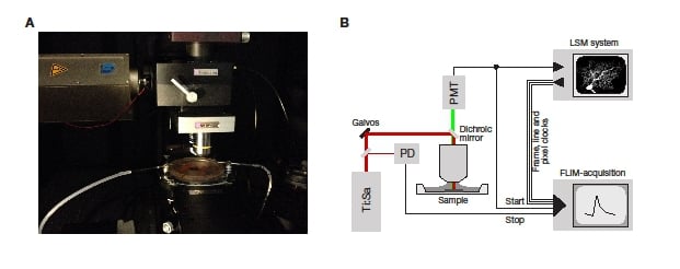
Figure 2: Implementation of a two-photon FLIM system. A: The microscope used for the work presented here. B: A schematic detailing the signal flow in an LSM FLIM system. The FLIM system receives inputs from the dectector (PMT) and the photodiode detecting the laser pulses (PD) to measure the fluorescence lifetime. In addition, it receives routeing inputs from the LSM system to allow the lifetimes to be assigned to the correct pixels.
Example experiment
To demonstrate the functionality of our system we used FLIM-FRET to monitor a conformational change in the NMDA receptor intracellular domain7.
Cultured dissociated hippocampal neurons were co-transfected with GluN1 subunits that were terminally tagged with either GFP or mCherry. In addition, the neurons were transfected with GluN2B subunits. Together these subunits should assemble to fully functional NMDA receptors. As GFP and mCherry form a FRET-pair, the fluorescence lifetime of GFP (as FRET donor) should be shorter in cells expressing receptors with both tags (Figure 3A). Indeed, spines in cells transfected only with GluN1-GFP showed a significantly longer GFP fluorescence lifetime (2,110 ± 4 ps, n = 711 spines) than spines in cells transfected with both GluN1-GFP and GluN1-mCherry (1,986 ± 6 ps, n = 470 spines; p < 0.0001; see Figure 3B). Using this difference in lifetime, it is possible to calculate the average distance between the two tagged subunits as 8.3 nm. This value is consistent with dimensions obtained by crystallography of single NMDA receptors11. This result demonstrates that we are able to perform reliable FLIM-FRET measurements.
Next, we bath applied NMDA to activate the tagged receptors (while also applying 7-chlorokyneuric acid to block current through the receptor). In cells expressing both GluN1-GFP and GluN1-mCherry, the lifetime of GFP fluorescence was significantly increased by NMDA application (see Figure 3C). This 52 ± 6 ps increase in fluorescence lifetime is indicative of a reduced FRET efficiency. The change matches an approximate 1 nm increase in the distance between GFP and mCherry (Figure 3C, bottom).
These results indicate that the system we present here is sensitive enough to detect conformational changes in neurotransmitter channels following application of a specific agonist.
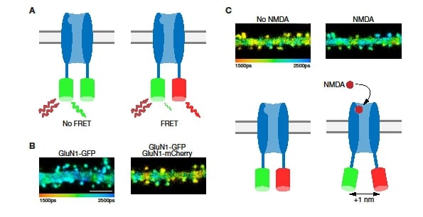
Figure 3: Measuring receptor subunit distances with FLIM-FRET. A: Schematic of a channel with only GFP-tagged subunits (left) and one with subunits tagged with both GFP and mCherry (right). Only receptors containing both tags are expected to show FRET (scale bar = 5 μm). B: Dendrites in neurons expressing only the GFP tag (left) show a longer GFP fluorescence lifetime than those in neurons expressing both tags (right). C: A dendritic branch before (left) and after (right) the application of NMDA. Note the change in fluorescence lifetime. Below each image is a cartoon model of the conformational change on NMDA binding that leads to the change in FRET efficiency.
References
1. Scanziani, M. & Häusser, M. Electrophysiology in the age of light. Nature 461, 930–939 (2009).
2. Becker, W. Advanced Time-Correlated Single Photon Counting Techniques. 81, (Springer, 2005).
3. Kaneko, H., Putzier, I., Frings, S. & Gensch, T. Determination of intracellular chloride concentration in dorsal root ganglion neurons by fluorescence lifetime imaging. Curr. Top. Membr. (2002).
4. Wilms, C. D., Schmidt, H. & Eilers, J. Quantitative two-photon Ca2+ imaging via fluorescence lifetime analysis. Cell Calcium 40, 73–9 (2006).
5. Jares-Erijman, E. A. & Jovin, T. M. FRET imaging. Nat Biotechnol 21, 1387–1395 (2003).
6. Dore, K., Labrecque, S., Tardif, C. & De Koninck, P. FRET-FLIM investigation of PSD95-NMDA receptor interaction in dendritic spines; control by calpain, CaMKII and Src family kinase. PLoS One 9, (2014).
7. Dore, K., Aow, J. & Malinow, R. Agonist binding to the NMDA receptor drives movement of its cytoplasmic domain without ion flow. Proc. Natl. Acad. Sci. U. S. A. 112, 14705–10 (2015).
8. Lakowicz, J. R. Principles of fluorescence spectroscopy. (Kluwer Academic/Plenum Publishers, 1999).
9. Levy, S. et al. SpRET: highly sensitive and reliable spectral measurement of absolute FRET efficiency. Microsc. Microanal. 17, 176–90 (2011).
10. Wallrabe, H. & Periasamy, A. Imaging protein molecules using FRET and FLIM microscopy. Curr. Opin. Biotechnol. 16, 19–27 (2005).
11. Lee, C.-H. et al. NMDA receptor structures reveal subunit arrangement and pore architecture. Nature 511, 191–197 (2014).
Other SciMethods you may find interesting...
SciMethods: Simultaneously recording from four neurons using PatchStar and MicroStar manipulators
SciMethods: Visual Stimulation of Retinal Explants on a Standard Multiphoton Microscope
SciMethods: Paired Blind Polytrode and Juxtacellular Recordings In Vivo
SciMethods: Controlling and Coordinating Experiments in Neurophysiology