A Deeper Look : More on Lasers
Introduction
Of all the topics that crop up in discussions with customers looking for multiphoton systems, the one regularly causing the most uncertainty is choosing the right laser or lasers for a new microscope. Given the price tag and the fact that a laser can make or break an experiment, this isn’t surprising. Complicating matters, both the range of applications and the number of available laser options have increased in recent years.
Two decades ago, for most users “multiphoton microscopy” really only meant “two-photon imaging”, which limited the laser requirements. At the same time, the laser selection was limited to a few mode-locked Ti:Sa laser models. More than anything the choice was down to the question of “hands-off” (e.g. Spectra-Physics Mai Tai or Coherent Chameleon) or “daily TLC needed” (e.g. Coherent Mira or Spectra-Physics Tsunami) and which supplier was able to provide the better deal.
In contrast, “multiphoton microscopy” today can refer to two-photon imaging, three-photon imaging, and two-photon photostimulation. All these approaches have very different laser requirements – and that is before you get into the details of individual experiments. This widening of laser requirements comes in parallel with more laser options becoming available. Ti:Sa lasers are still widely used, but one-box OPOs (optical parametric oscillators) with their expanded tuning range such as the Coherent Discovery NX, Light Conversion Cronus-2P, or Spectra-Physics Insight X3 have replaced them in many cases. At the same time fixed-wavelength fiber lasers have become available in several key wavelengths, in particular 920 nm for excitation of eGFP. These ultrafast lasers tend to have high repetition rates (20 to 100 MHz), which, as we will see below, are not appropriate for all techniques. Thus, lasers with lower repetition rates (typically <2 MHz) are also becoming increasingly common in multiphoton labs.
Which all leads to two big questions:
- Which of the different options is the best fit for my experiments?
- What makes one laser a better fit for those experiments than other lasers?
In this article we aim to develop a better understanding of the latter, putting you in a position to better evaluate the former.
For reasons of clarity, we will mainly focus on two-photon excitation, mentioning three-photon explicitly when it is considered. Many of the core concepts apply to both.
Back to basics
Approaching this topic, it seems helpful to start by taking a big step back: Why do we use the lasers that we do for two-photon imaging?
Two-photon excitation requires two individual photons to interact with a single fluorescent molecule at the same time. For this interaction to be sufficiently likely, a very high density of photons is required. In material sciences this was achieved using high laser powers (>10W), which would destroy almost any biological sample instantaneously. The way around this is simple: instead of continuously applying the power levels required for efficient two-photon excitation, they are instead applied in very short bursts, or pulses. For pulse durations in the 100 – 150 fs range, the power level achieved in these pulses (i.e. the peak power, Ppeak) is several orders of magnitude higher than the average power, allowing average powers to be used that are compatible with live biological tissue.
The interplay of average power, peak power, pulse width, laser repetition rate and pulse energy are at the heart of selecting the best laser for given methods. At times we find that it can be easy to get a bit lost in these different parameters. To help avoid that happening we will give a phenomenological description of these parameters and how they link in the following paragraphs. We will use a Ti:Sa laser as an example – for no other reason than that these lasers are widely used and can run in a pulsed and a non-pulsed (continuous wave) state. The same concepts apply to other lasers.
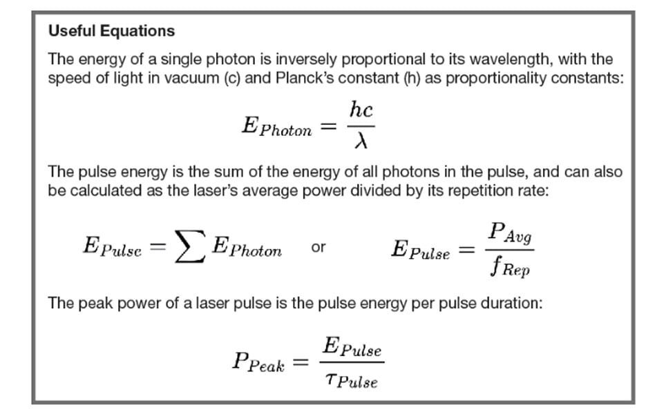
When a (Ti:Sa) laser is not pulsing, a state referred to as “continuous wave (CW) emission”, it will emit a steady power level over time. Assuming this laser is set up to emit 1 W, then no matter how short the time window the laser power is measured in, it will always be 1 W – the laser’s energy is spread evenly over time. If this same laser is brought to pulsing (i.e. the Ti:Sa laser is mode-locked), the power measured by a standard power meter (i.e. the average power) will remain the same, as power meters are slow and average power over time. The actual emission happens only in very short pulses (e.g. 100 fs) with relatively long gaps between them – for a typical Ti:Sa laser there are 80 million pulses per second (i.e. a repetition rate of 80 MHz, resulting in 12.5 ns between pulses). This spreads the laser’s energy unevenly over time, with each pulse having a fixed energy (the pulse energy) and no energy being emitted between pulses. The pulse energy (EPulse) is the sum of the energy of all photons in a laser pulse and can be calculated as the ratio of the average power (PAvg) over the laser repetition rate (frep). From this relationship (see the “Useful Equations” box below), it becomes clear that the higher the average power and the lower the repetition rate, the higher the pulse energy will be. In the case of our Ti:Sa laser with 1 W average power and 80 MHz repetition rate this would be 12.5 nJ.
Knowing the pulse energy is the first step to determining the laser power during the pulse (i.e. the peak power, PPeak): this is simply the pulse energy divided by the pulse duration. So, while the pulse energy is proportional to the number of photons in a laser pulse, the peak power is proportional to the density of photons in the laser pulse. In the case of our hypothetical Ti:Sa laser, this corresponds to pulse energy of 125 kW.
Looking at this example, the power (pun not intended, but appreciated) of using a pulsed laser becomes apparent: a pulsed 1 W average power laser readily achieves a peak power that is five orders of magnitude higher than in a 1 W continuous wave laser, while the heat load output by the laser remains stable at 1 W. So, when using a pulsed laser, two-photon excitation does not require power levels incompatible with biological tissue (e.g. 50 mW of average power from a pulsed Ti:Sa laser rather than the 15 W of a non-pulsed Ti:Sa laser required to achieve the same level of fluorescence).
How do all these parameters play together in determining the efficiency of two photon excitation? We look at that next.
Two-Photon Excitation Efficiency
What determines the intensity of two-photon excited fluorescence? Most multiphoton microscopists will immediately answer with “the laser power”, followed by “the fluorescence intensity increases with the square of the laser power”. That answer is correct, but as we saw above not sufficient and of little help when choosing and setting up a laser.
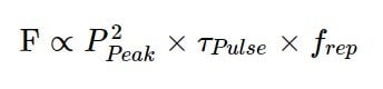
A first step towards a robust measure of the “two-photon excitation capability of a laser” is to consider the peak power. The instantaneous ability to excite fluorescence is indeed directly dependent on the square of the peak power; however, actual image brightness is determined by the time-integrated fluorescence. Moving from the instantaneous fluorescence excitation capability to the effect of the laser on the actual fluorescence thus requires two other factors to be considered: pulse width and repetition rate.
For a given peak power, the longer a laser pulse is, the longer the sample is exposed to excitation. So, the fluorescence intensity is proportional to the product of peak power and pulse width:
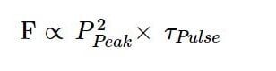
Which explains the fact that two-photon excitation scales linearly and not squarely with the pulse width – so all other things being equal, a doubling of the pulse width should lead to a halving of the fluorescence. A fact that is not always appreciated.
Finally, the time-integrated fluorescence will increase with the number of pulses a sample is exposed to in that time. This is where the repetition rate comes into play. Extending the equation above then yields:
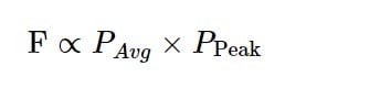
For those who want a shortcut, this can be simplified to:
A more detailed discussion of this can be found in this excellent review by Warren Zipfel, Rebecca Williams, and Watt Webb, but the resulting equation in that review is equal to the one above.
For three-photon excitation, the same basic concepts apply, but the instantaneous excitation is proportional to the cube of the peak power. Therefore, the relationship of pulse width to three-photon excited fluorescence is square and not linear.
Equipped with this background, we can go back to the core question: which laser is best suited for which types of experiments? There are two main limitations that play into this choice:
- The sample must be able to tolerate the imaging.
- The resulting laser requirements need to match an existing and ideally reasonably available laser.
The initial limitation from which all else follows is that the sample must be able to tolerate the imaging. In multiphoton microscopy, the primary damage mechanism is tissue heating, chiefly driven by absorption of laser light by the sample (mainly by the water in the tissue). The amount of absorption is dependent on the average power and wavelength of the laser applied to the tissue (a combination often referred to as the “heat load”). We will look at this in a bit more detail in the next section.
The Heat Load Limit and Working Around It
To state the obvious: biological tissue and processes are temperature sensitive. If the temperature of an organ is raised above its physiological temperature, there will initially be (reversible) changes to the physiology of the tissue, followed by irreversible structural damage at higher temperatures. The temperature changes that can be tolerated strongly depend on the organism and tissue being studied, but for most mammalian tissue this will typically be in range of just one to four degrees Celsius.
The relationship between power level and temperature increase depends on a range of parameters. First and foremost, the laser wavelength being used will be the main determining factor as light absorption by water is highly wavelength dependent (see Figure 1). At wavelengths with higher absorption, the power limit will be lower, so when imaging with 920 nm excitation light, the power limit will be much higher than at 1700 nm.
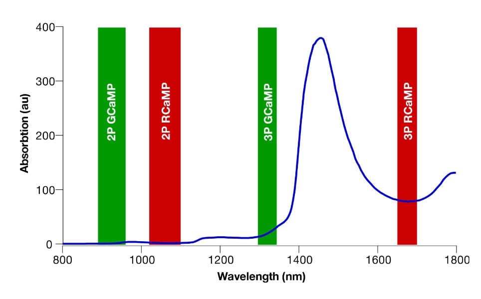
For the mouse brain, typically found limits are 200 – 250 mW at 920 nm (see Podgorski and Ranganathan, 2016) and 125 – 150 mW at 1320 nm (see Wang et al., 2020).
This “biocompatibility limit” is an ideal starting point for determining which laser parameters will work in your sample. The next question is how much excitation capability is needed for the planned experiments. This will vary for different types of experiments and tends to be only rarely determined and described quantitatively. As an example, video-rate two-photon imaging of GCaMP will have different excitation requirements than three-photon imaging of the same indicator, and both will differ substantially from two-photon optogenetics using an SLM to generate spots that are scanned over cell bodies.
At the core, choosing the correct laser parameters is an exercise of determining the maximum biocompatible average power for a given sample, and then determining how to distribute that power in time to achieve the required excitation capability. “Distributing in time” factors in both repetition rate and pulse width.
This is best explained with an example: In two-photon optogenetics, stimulation of a single neuron to fire an action potential using a spiralling spot will require 6 mW of average laser power from a laser with a 2 MHz repetition rate and a pulse width of 250 fs (Russell et al., 2022). Using the equations above, we can quickly calculate that this corresponds to 12 kW peak power and thus 72 W2 two-photon excitation capability. Using a typical Ti:Sa laser, with a repetition rate of 80 MHz and 120 fs pulse width, the same excitation capability would require 26 mW. For a single cell that is a power level that is easily tolerated by a mouse brain. However, if a researcher wishes to scale up from a single cell to 100 cells at the same time, the Ti:Sa laser would need to provide 2.6 W to the sample, a power level that will undoubtedly cause damage to the sample after all but the shortest exposures. In comparison, the lower repetition rate laser would need to provide only 600mW, which is generally well-tolerated for intermittent burst of stimulation.
Those calculations bring us to the second element in the list of limitations: the required laser parameters must be achievable by a readily available laser. To achieve 2.6 W out of the objective in even the most efficient multiphoton microscope will require over 6 W of output from the laser. At 80 MHz repetition rate and 120 fs pulse width that is simply not achievable at a reasonable price (if it is commercially available at all).
Phototoxicity
Thus far, we have focused on damage caused by tissue heating for the simple reason that in multiphoton imaging this is often the most obvious form of photodamage. Heating is a linear process affecting the entire tissue volume exposed to the excitation light. On the other hand, phototoxicity (i.e. molecules in excited states triggering chemical reactions with cellular components, damaging the cell) is primarily limited to the focal volume in multiphoton microscopy. In contrast, during one-photon excitation the entire volume exposed to the excitation light (which is of a much shorter wavelength, and thus much higher energy) will be prone to phototoxicity. Counter to what is often assumed, in the focus phototoxicity is more pronounced in multiphoton than one-photon microscopy.
Some work has been done to identify energy or power levels at which phototoxicity becomes an issue in two- and three-photon microscopy, and, anecdotally, the threshold is similar, at around 8 to 10 nJ at the focus. Importantly, this is lower than the intensity emerging from the objective, as substantial levels of light are lost through scattering and absorption prior to reaching the focus.
One important fact to consider here is that phototoxicity in multiphoton imaging is very non-linear. Under typical two-photon conditions, the damage is caused by a range of different processes, some of which are not second order (i.e. two-photon), but higher orders, up to fifth. On average they appear to follow a power law on the order of 2.5 (Hopt & Neher, 2001). This explains why increasing peak power leads to more fluorescence, but a greater proportional increase in phototoxicity.
While in most multiphoton applications the damage caused by heat is expected to dominate, it is worth keeping phototoxicity in mind – especially when considering two-photon photostimulation or three-photon imaging.
Final thoughts
So where does this leave us? Well, ideally, we would all like to have very bright fluorescence while not heating or damaging the tissue with laser light. However, as discussed above, those two are mutually exclusive. Thus, choosing the right laser for a given experiment will always be a matter of balance and compromise between these factors.
But there are also other factors that play into this compromise. Indeed, as some readers may have noticed, we glossed over the fact that the repetition rate of the laser will impact the fastest achievable imaging speed. With a resonance scanner, each pixel is exposed to the laser on average around 125 ns. For a Ti:Sa at 80 MHz repetition rate, that corresponds to 10 laser pulses. For a fibre laser with 10 MHz repetition rate, it would correspond to 1.25 pulses, meaning that on average three pixels are exposed to one pulse each, followed by a fourth pixel exposed to two pulses. In the case of a 1 MHz repetition rate laser, only every eighth pixel would be exposed to an excitation laser pulse. Clearly, the last two cases are useless for quantitative imaging. This becomes relevant for three-photon imaging, where efficient excitation tends to require repetition rates around 0.3 to 4 MHz, depending on required imaging depth. Fast fluorescence indicators that require tens of frames per second will be challenging to use in these experiments.
The biggest take away from all this should be that the microscope is not what determines which laser is required on a setup. Instead, the experiments that the microscope will be used for are crucial to deciding this.
Introduction
Of all the topics that crop up in discussions with customers looking for multiphoton systems, the one regularly causing the most uncertainty is choosing the right laser or lasers for a new microscope. Given the price tag and the fact that a laser can make or break an experiment, this isn’t surprising. Complicating matters, both the range of applications and the number of available laser options have increased in recent years.
Two decades ago, for most users “multiphoton microscopy” really only meant “two-photon imaging”, which limited the laser requirements. At the same time, the laser selection was limited to a few mode-locked Ti:Sa laser models. More than anything the choice was down to the question of “hands-off” (e.g. Spectra-Physics Mai Tai or Coherent Chameleon) or “daily TLC needed” (e.g. Coherent Mira or Spectra-Physics Tsunami) and which supplier was able to provide the better deal.
In contrast, “multiphoton microscopy” today can refer to two-photon imaging, three-photon imaging, and two-photon photostimulation. All these approaches have very different laser requirements – and that is before you get into the details of individual experiments. This widening of laser requirements comes in parallel with more laser options becoming available. Ti:Sa lasers are still widely used, but one-box OPOs (optical parametric oscillators) with their expanded tuning range such as the Coherent Discovery NX, Light Conversion Cronus-2P, or Spectra-Physics Insight X3 have replaced them in many cases. At the same time fixed-wavelength fiber lasers have become available in several key wavelengths, in particular 920 nm for excitation of eGFP. These ultrafast lasers tend to have high repetition rates (20 to 100 MHz), which, as we will see below, are not appropriate for all techniques. Thus, lasers with lower repetition rates (typically <2 MHz) are also becoming increasingly common in multiphoton labs.
Which all leads to two big questions:
- Which of the different options is the best fit for my experiments?
- What makes one laser a better fit for those experiments than other lasers?
In this article we aim to develop a better understanding of the latter, putting you in a position to better evaluate the former.
For reasons of clarity, we will mainly focus on two-photon excitation, mentioning three-photon explicitly when it is considered. Many of the core concepts apply to both.
Back to Basics
Approaching this topic, it seems helpful to start by taking a big step back: Why do we use the lasers that we do for two-photon imaging?
Two-photon excitation requires two individual photons to interact with a single fluorescent molecule at the same time. For this interaction to be sufficiently likely, a very high density of photons is required. In material sciences this was achieved using high laser powers (>10W), which would destroy almost any biological sample instantaneously. The way around this is simple: instead of continuously applying the power levels required for efficient two-photon excitation, they are instead applied in very short bursts, or pulses. For pulse durations in the 100 – 150 fs range, the power level achieved in these pulses (i.e. the peak power, Ppeak) is several orders of magnitude higher than the average power, allowing average powers to be used that are compatible with live biological tissue.
The interplay of average power, peak power, pulse width, laser repetition rate and pulse energy are at the heart of selecting the best laser for given methods. At times we find that it can be easy to get a bit lost in these different parameters. To help avoid that happening we will give a phenomenological description of these parameters and how they link in the following paragraphs. We will use a Ti:Sa laser as an example – for no other reason than that these lasers are widely used and can run in a pulsed and a non-pulsed (continuous wave) state. The same concepts apply to other lasers.
When a (Ti:Sa) laser is not pulsing, a state referred to as “continuous wave (CW) emission”, it will emit a steady power level over time. Assuming this laser is set up to emit 1 W, then no matter how short the time window the laser power is measured in, it will always be 1 W – the laser’s energy is spread evenly over time. If this same laser is brought to pulsing (i.e. the Ti:Sa laser is mode-locked), the power measured by a standard power meter (i.e. the average power) will remain the same, as power meters are slow and average power over time. The actual emission happens only in very short pulses (e.g. 100 fs) with relatively long gaps between them – for a typical Ti:Sa laser there are 80 million pulses per second (i.e. a repetition rate of 80 MHz, resulting in 12.5 ns between pulses). This spreads the laser’s energy unevenly over time, with each pulse having a fixed energy (the pulse energy) and no energy being emitted between pulses. The pulse energy (EPulse) is the sum of the energy of all photons in a laser pulse and can be calculated as the ratio of the average power (PAvg) over the laser repetition rate (frep). From this relationship (see the “Useful Equations” box below), it becomes clear that the higher the average power and the lower the repetition rate, the higher the pulse energy will be. In the case of our Ti:Sa laser with 1 W average power and 80 MHz repetition rate this would be 12.5 nJ.
Knowing the pulse energy is the first step to determining the laser power during the pulse (i.e. the peak power, PPeak): this is simply the pulse energy divided by the pulse duration. So, while the pulse energy is proportional to the number of photons in a laser pulse, the peak power is proportional to the density of photons in the laser pulse. In the case of our hypothetical Ti:Sa laser, this corresponds to pulse energy of 125 kW.
Looking at this example, the power (pun not intended, but appreciated) of using a pulsed laser becomes apparent: a pulsed 1 W average power laser readily achieves a peak power that is five orders of magnitude higher than in a 1 W continuous wave laser, while the heat load output by the laser remains stable at 1 W. So, when using a pulsed laser, two-photon excitation does not require power levels incompatible with biological tissue (e.g. 50 mW of average power from a pulsed Ti:Sa laser rather than the 15 W of a non-pulsed Ti:Sa laser required to achieve the same level of fluorescence).
How do all these parameters play together in determining the efficiency of two photon excitation? We look at that next.